This document explains the math used in the L and Rs part of atlc2. Actually, this was a planning document used by the author of atlc2, and the program follows it very closely. Criticism is welcome.
(Solving these equations is straight-forward, but first you must decide which variables are knowns and which are unknowns.)
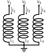
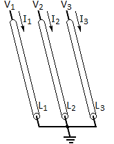
The same three equations would apply. But the self inductance of an infinite, unpaired wire wire is infinite. Even its "per meter" inductance is infinite. But if we require that the currents are paired such that I1+ I2+ I3 = 0, then there will be no radiation and the circuit is solvable.
With no net current, there is no magnetic field except very close to the wires. This is a hint that the self inductance terms play no role.
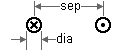
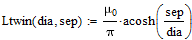
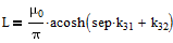
Now suppose the wires are each 1 meter long, equal in diameter and resistivity, and the frequency is 10-10 Hz. Capacitive effects can be disregarded in such short stubs, but transmission line equations can be used to find the inductances. The usual formula for twinlead inductance is :
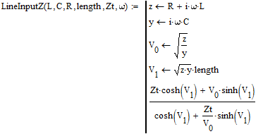
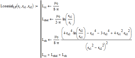
If the length = 1 meter and the frequency = 10-10 then effectively cosh(V1) = 1 and sinh(V1) = V1. If Zt = 0 then this function simplifies to :
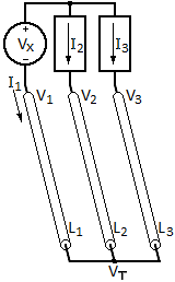
A superposition argument will be used to apply the two-wire transmission line formula. Inactive voltage sources must be set to 0 Volts and 0 Ohms, which is a problem since it would allow current in more than just two wires. So we shall switch to constant current sources and investigate the resulting voltages. Inactive current sources become infinite impedances.
Since I1+ I2+ I3 = 0, there is no ground current at the termination. Let the termination voltage be VT, which is probably close to ground but not necessarily at ground.
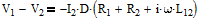
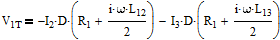
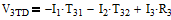
According to the above transmission line formula, the I2 superposition current will produce an input voltage :
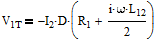
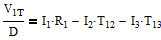
For very short stubs V1 - VT will be exactly half of V1 - V2 if R1 = R2. Let V1T = V1 - VT. In the general case :
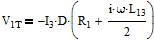
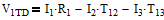
V1TD is the superposition sum of voltages on wire 1 that result from the forced currents I2 and I3. VX will never contribute since it is in series with infinite impedances.
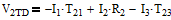
These resemble the original three equations. Note that the self inductance terms are now gone. There is no inductance except from paired conductors. It is valid to view the circuit as a superposition of 2-wire transmission lines. Since these 2-wire lines do not radiate, neither does the superposition.
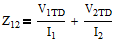
After solving this set of equations, suppose I3 turns out to be zero or insignificant. Then the circuit could be characterized by the input impedance of the other two wires, which would be :
It is common to want this impedance expressed as a "per meter" quantity. To do this, just set D = 1. If D had been 1 from the start, the same result would have been obtained. The only purpose of D is to make the example physically understandable. (The math describes a very short stub, not a 1 meter stub.)
In the next example, D will be omitted from the math. Its inclusion would not change anything.
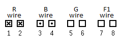
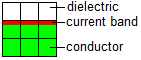
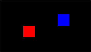
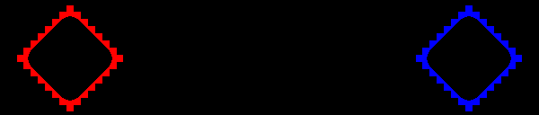
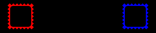
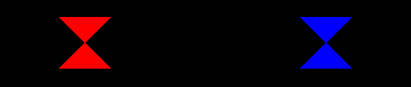
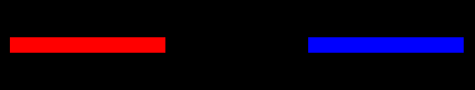
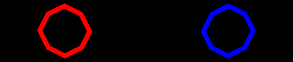
R wire: red, with voltage VR
B wire: blue, with voltage VB
G wire: green, with voltage VG
F1 wire: floater #1, with voltage VF1
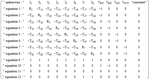
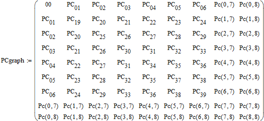
Atlc2 has a large array called the Coefficient Pool that holds all the equations. The array would be square except that there is an additional column for the constants. Each row is an equation, and each column is for an unknown. Each coefficient is two 8-byte numbers: real and imaginary. For 13,600 equations this array will occupy 3 gigabytes of RAM.
The total number of equations is p + r + b + g + f, where :
p is exactly the number of conductor pixels.
r is 1 if there is a +1 wire (red), 0 otherwise.
b is 1 if there is a -1 wire (blue), 0 otherwise.
g is 1 if there is a 0 wire (green), 0 otherwise.
f is the number of colors used for floating wires.
note 1: This equation will be VRT - VGT = 1 if VBT is missing, VGT - VBT = 1 if VRT is missing.
note 2: This equation will be present only if the R, B, and G wires are all present.
note 3: This equation will be missing if there is no corresponding wire.
ZPM is exact if there is no third current, and a good approximation if the third current is very small. Otherwise L and RS are undefined, but the program will report them anyway, so use them at your own peril.
There are some problems with the usual formula for twinlead inductance :
1. It assumes round wires, not square pixels.
2. It assumes the conductor separation is not too small.
3. It assumes the frequency is high.
The atlc2 general method assumes that the current is evenly distributed over the face of the pixel. In effect, this is the low frequency case.
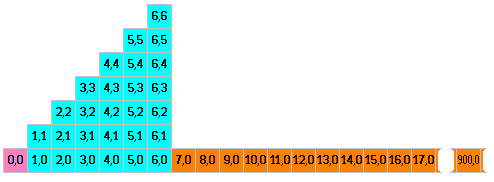
For calculating pool coefficients, atlc2 works differently for close and far pairings :
1. A table-lookup is used when the separation is very small. These are the pink-cyan cases below.
2. A formula resembling the usual formula is used for larger separations, the pink-orange cases.
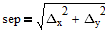
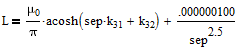
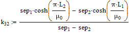
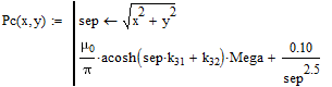
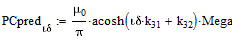
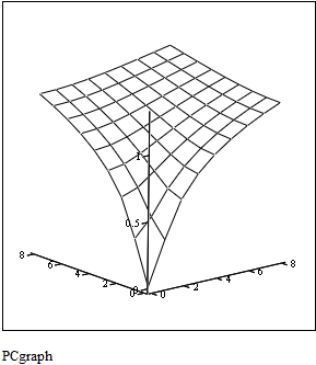
This inductance formula is for the pink square paired with one of the orange squares, but it is used for all squares farther than 6 from the pink square. (Atlc2 assumes that rotation of the square pixels does not have a significant effect at the larger separations.) ΔX and ΔY equal the integer coordinates of the orange square.
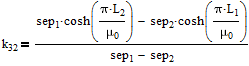
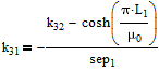
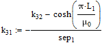
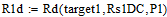
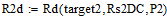
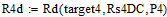
I decided it best to derive k31 and k32 from the inductances for pixel 14,0 and pixel 900,0. It is not hard to show that :
Rs: a rough guess :
If the D.C. resistance of each pixel is used to build the Coefficient Pool then the computed Rs will be accurate to ±1% when the skin depth is at least 30 times the pixel width.
In other words, if the drawing had too few pixels, the computed L would be noisy but roughly correct. But the computed Rs would be seriously low. As described so far, the current is assumed to be evenly distributed across the face of the pixel. But if, for example, only one fifth of each pixel is carrying current then the true Rs would be five times what the program would report.
Estimating Rs at high frequencies :
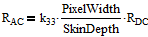
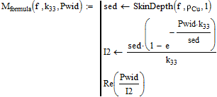
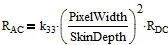
The resistance of a pixel is its resistivity divided by its area. If the A.C. effective area is used then L and Rs will be accurate, and many fewer pixels are needed for an accurate Rs. The A.C. area can be estimated from the predicted skin depth. So at the highest frequencies L and Rs uses this formula :
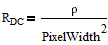
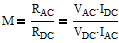
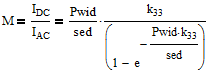
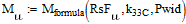
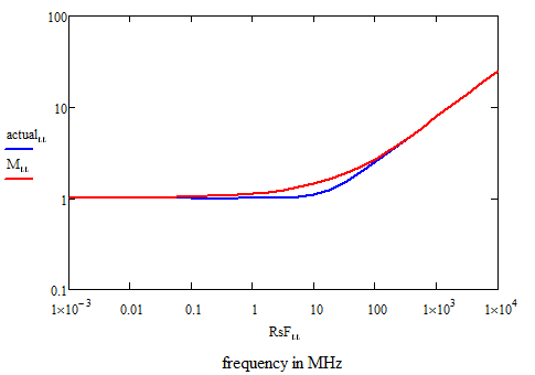
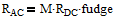
This accurately portrays the resistance when the current is concentrated along a side of the pixel. But it is wrong at low frequencies. RAC must never be less than RDC. For all frequencies we must find the function M, where :
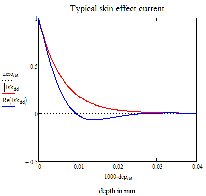
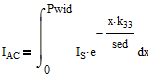
I(x) is the current at depth x
sed is the skin effect depth. sed is a constant obtained from the common skin effect depth formula.
IS is the current at the surface.
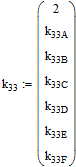
k33 is a constant to be determined.
(This rough formula, which ignores phase-shifted currents, is good enough for the moment.)
If the conductor is viewed as resistors in parallel, then we can find M using Ohm's law:
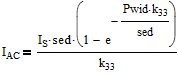
If the current is always IS at the surface then VAC = VDC, and they drop out. Integration is to the depth of 1 pixel, Pwid. These simplify to:
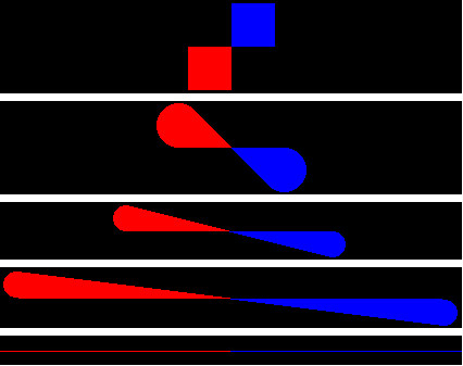
The red plot below shows a typical M versus frequency. But the M formula is approximate. Simulations show that the truth tends to follow the blue plot below.
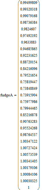
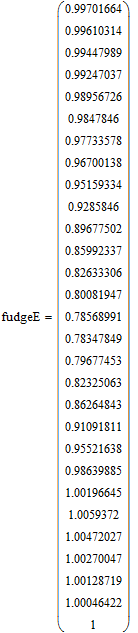
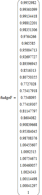
"fudge" is a function, whatever is necessary to produce the correct AC resistance. The fudge function is found using numerical methods. A typical fudge function looks like this:
When the current is forced into just a corner of a pixel, this equation would seem more appropriate :
But in experimenting, I found that the true power is always less than 2. Here are some cases I found:
"power" refers to how the resistance changes in the centermost two pixels, but also the whole structure at middle frequencies. (This will be explained better later.)
But these cases are peculiar in that the conductors are extremely close. When they are further apart, the power is always 1.00. (I was not able to find a contradictory example. It might be said that, when the conductors are close together, the skin effect is an attractive force very concentrated. When they are far apart, it is a mostly repulsive force rather diffuse.)
Presently atlc2 assumes the power is always 1.00, as if the conductors are far apart. So the Rs value computed by atlc2 will be wrong when they are nearly touching. (The L value is still quite accurate.)
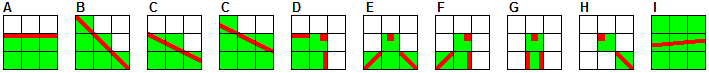
Atlc2 concerns itself with the following nine cases. Each case seeks the resistance of the center pixel, given its 8 neighbors :
There are other cases, but they are either rotations of these 9, or cases unlikely to appear in a well constructed simulation and not likely significant if they do.
Case A is the most typical case. Cases B and C could be corner pixels, but atlc2 will assume they are part of a flat or curved surface. Cases D and E are 90o corners, and F is a 45o corner. A well thought out Usermap probably would not contain instances of cases G or H. All other cases are treated as interior pixels.
Case I is for all interior pixels. The skin effect current dies away exponentially with depth. So the A.C. effective area of interior pixels is likely about the same as that of typical surface pixels. I found that results are most accurate when the resistance of each interior pixel is the same as the closest surface pixel.
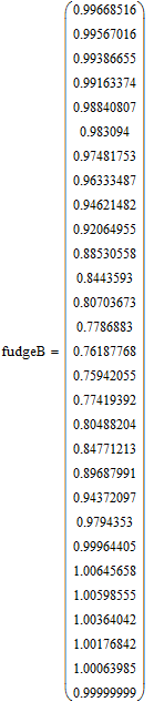
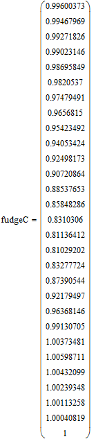
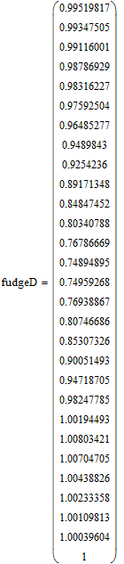
The fudge function and k33 are different for each of the 9 cases. I shall call them :
k33A, k33B, k33C, ...
fudegA, fudgeB, fudgeC, ...
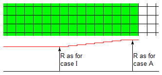
Good results are obtained when the resistances of pixels are tapered by depth. Pixels within 8 pixels of the surface are tapered from the surface value (such as case A) to the interior value (case I).
Because of this tapering method, the actual values of the constants k33I and fudgeI have minuscule effect at low frequencies and no effect at all at high frequencies. So atlc2 uses the case C constants for case I.
If you need an accurate Rs prediction, try to avoid employing cases G and H. The geometry of these cases is too unspecific to predict what should happen. Atlc2 uses the case C constants for cases G and H.
The next section describes the techniques used to determine the constants needed by atlc2. These constants include all the pixel inductances, k31 through k33, and the fudge functions.
I began by finding each L using C and Gp. This is good but not perfect since C and Gp cannot produce a low frequency result. But using these values as a starting point, L and Rs can be used to find better values for each L. This can be repeated until all the values stabilize, a "successive approximations" solution. Each iteration requires running L and Rs 40 times.
I added to atlc2 a feature that would automatically run L and Rs 40 times and record the 40 inductances in a single file easily loaded by Mathcad. The 40 internally generated bitmaps portray these cases:
8 pixel 8,0
9 pixel 9,0
10 pixel 10,0
11 pixel 11,0
12 pixel 12,0
13 pixel 13,0
14 pixel 14,0
15 pixel 15,0
16 pixel 16,0
17 pixel 17,0
18 pixel 900,0
19 pixel 1,1
20 pixel 2,1
21 pixel 3,1
22 pixel 4,1
23 pixel 5,1
The conductor pixel total can be set from the keyboard before the run. The frequency is always 1 Hz.
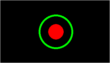
In choosing such inductances experimentally, it is necessary to have a standard for comparison. This becomes the feedback that makes successive approximations work. I chose this coaxial cable as a standard :
2mm center conductor diameter, copper.
4mm shield inner diameter, dielectric = vacuum
4.5mm shield outer diameter, copper.
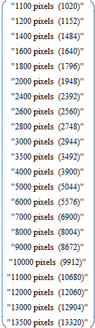
atlc2 will most accurately draw the standard coax when the requested "Total conductor pixels" is any of these : 1640, 2560, 3692, 5044, 6600, 8348, 10324, 12524, 14856, 17432, 20220, 23264, and 26388. These numbers are good for very high frequencies and very low frequencies, but not transitional frequencies.
Each iteration in the generation of the constants proceeds as follows:
1. The atlc2 automated procedure is run. This produces 40 inductances in a file.
2. The atlc2 source code is edited to place the 40 constants in the "ProposedConstants" array.
3. Atlc2 is recompiled. (Atlc2 is forbidden to have runtime files.)
4. When atlc2 begins running, it first creates the "ActualConstants" array.
At first I created the ActualConstants this way :
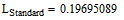
P is the theoretical inductance of the standard coax.
Q is the computed inductance of the standard coax, taken from ProposedConstants[0]
for x := 0 to 39 do ActualConstants[x] := ProposedConstants[x];
ActualConstants[14] := ProposedConstants[14] * P / Q;
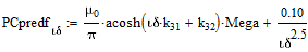
The new term improves the inductances of pixels 7,0 through 11,0, making them match the computed values more closely. The constants in the new term were found by hand. The effect of this new term is extremely small, about 1 part in 2000 for typical L and Rs runs.
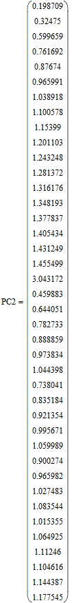
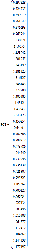
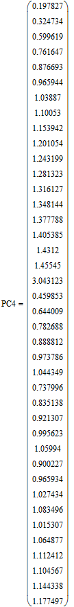
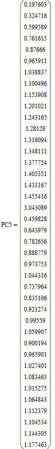
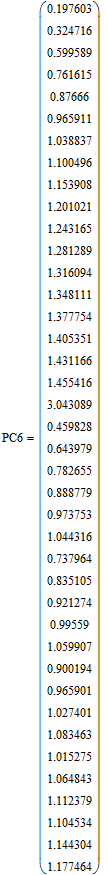
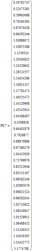
Each of the statements below fetches data from a file and loads it into an array. The PC0 data file was made by typing in C and Gp results. Then each other file was created by L and Rs using the data from the file immediately above it.
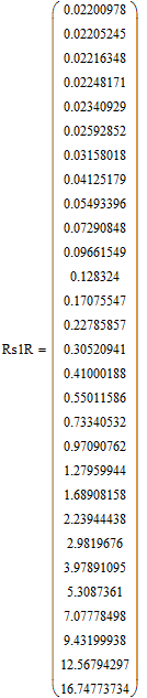
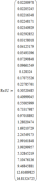
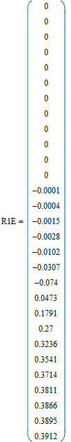
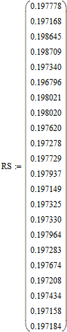
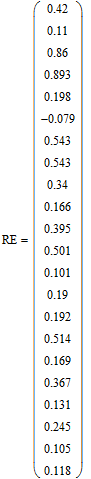
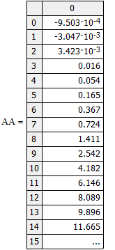
Atlc2 now uses the constants from the PC7 file. With these constants coded into it, L and Rs will produce these results for the standard coax :
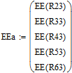
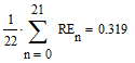
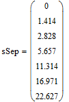
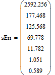
(I ran L and Rs 22 times and hand-typed the results into the RS array below.)
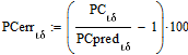
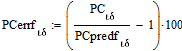
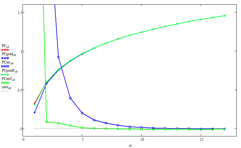
This graph shows the error that existed before the new term was added to the pixel inductance formula. (L in μH, error in %, blue: without correction, green: with correction, red: target from simulation.)
(Keep in mind, the formula is used only for distances greater than 6.)
Although not a proof, the results above suggest that the best accuracy L and Rs can achieve for curved surfaces is better than one half of 1 % for L values. Even with a low pixel count it was never as bad as 1 %.
(I think the average offset being non-zero is the result of a diameter flaw in the way atlc2 draws circular objects.)
In the following discussion, "SkinFix" refers to atlc2's ability to improve Rs by calculating the A.C. effective area of pixels. So "SkinFix disabled" means that current is always distributed evenly over the entire pixel.
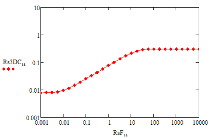
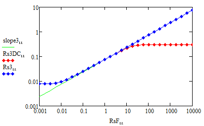
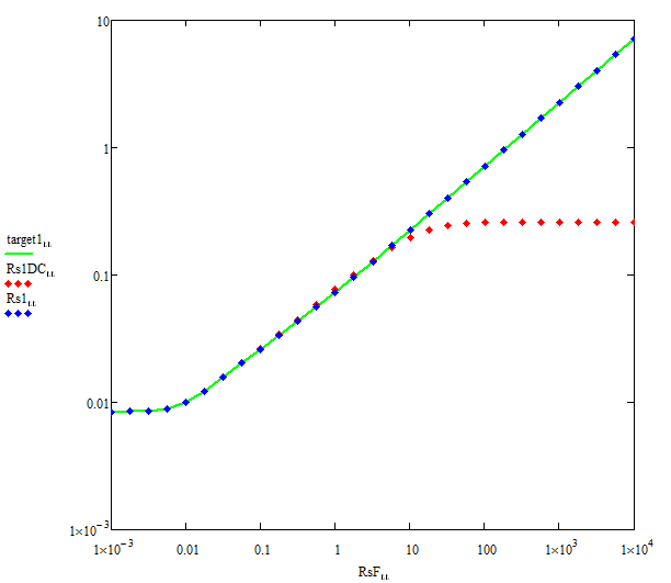
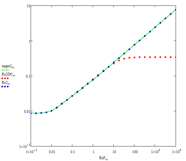
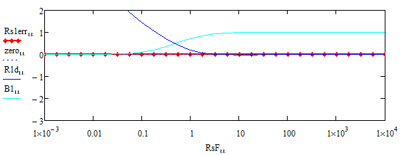
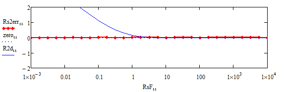
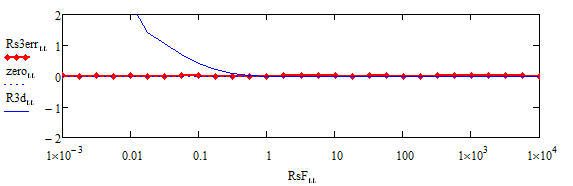
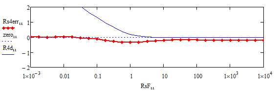
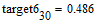
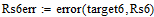
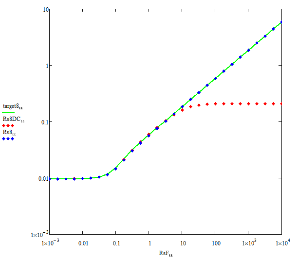
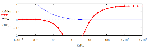
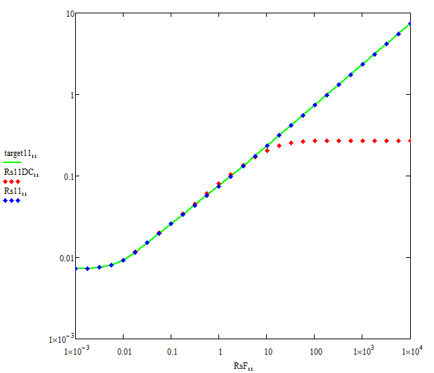
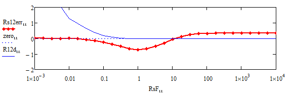
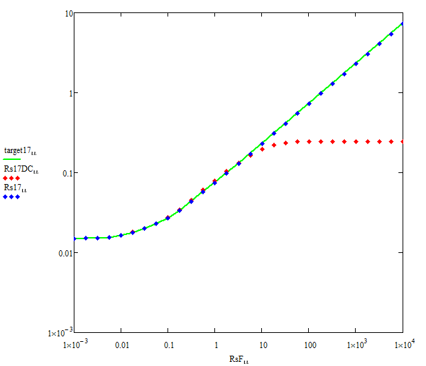
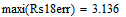
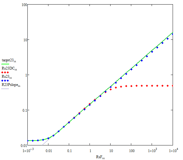
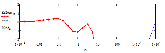
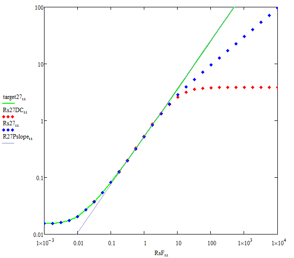
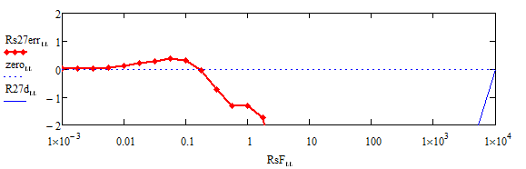
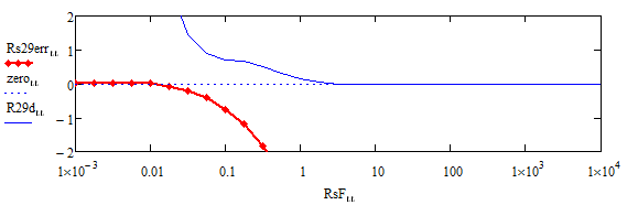
If L and Rs is run with SkinFix disabled, a graph of Rs versus frequency will usually look like this :
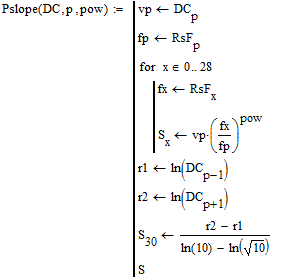
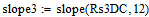
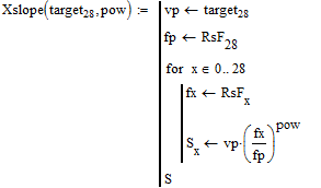
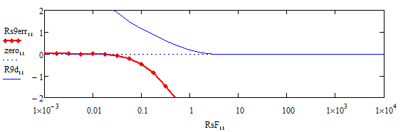
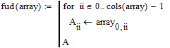
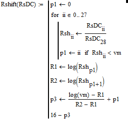
 creates a line passing through point p and having the slope designated by
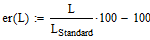
  . Then it measures the actual slope using the two points on either side of point p, and outputs that value as element 30.
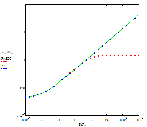
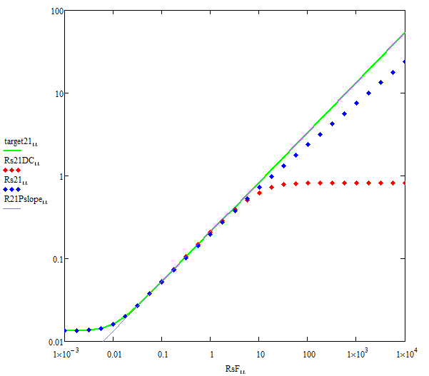
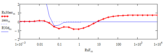
There are three regions. At very low frequencies, all the pixels have equal currents. At middle frequencies, the skin effect is eliminating the current from the central pixels. At very high frequencies, Rs levels off because the conduction path is whole pixels, and the pixels are too big. This level-off is wrong. The blue plot below shows SkinFix enabled.
If SkinFix is enabled, the conduction path continues to shrink, and the plot continues to rise. There should be no variation in the way it rises. It should continue to be a straight line. (In most cases the straight line would be an obvious square root plot if the axes were linear. In other cases the line is straight because the examples were chosen such that the shape of the current distribution does not change with frequency other than a simple rescaling.)
If k33 is chosen correctly, the blue line will be straight. If the fudge function is chosen correctly then there will be no graphical evidence of a transition from the middle to the highest frequencies.
The determination of these constants proceeded through the following steps :
Each of the 6 steps above were performed using the following procedure :
Thereafter, atlc2 will determine the fudge function value by interpolating (or extrapolating) the values found by the above procedure.
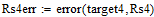
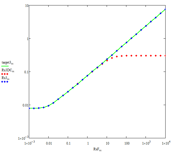
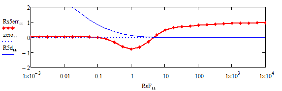
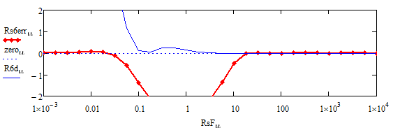
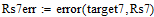
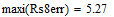
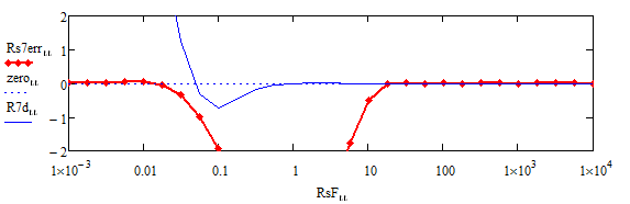
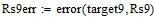
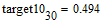
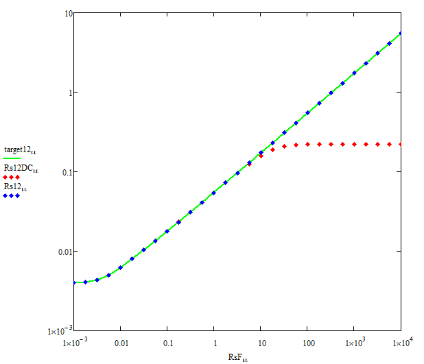
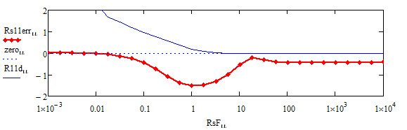
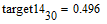
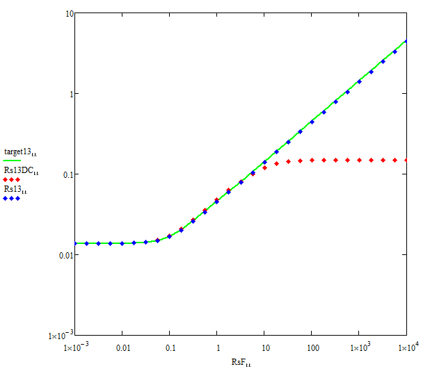
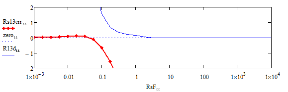
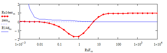
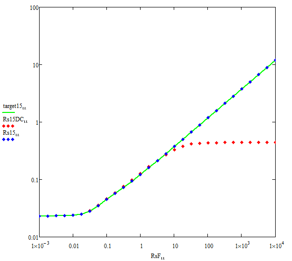
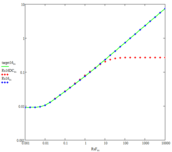
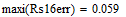
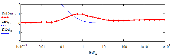
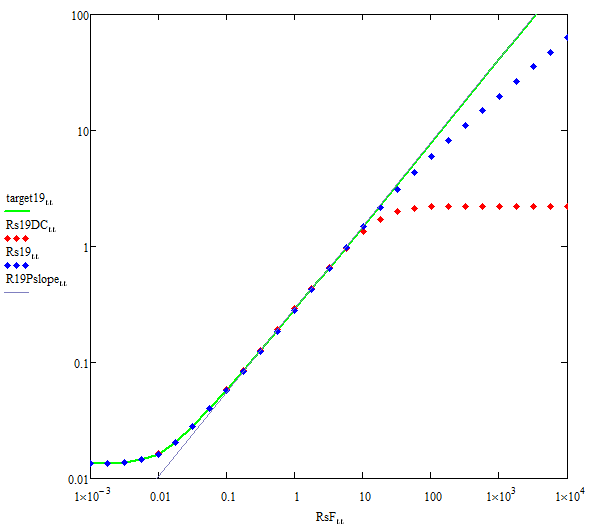
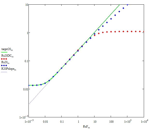
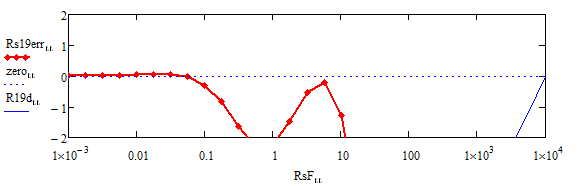
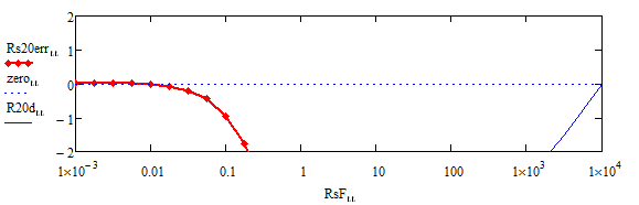
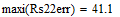
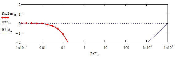
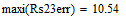
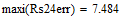
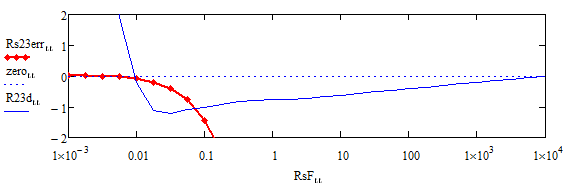
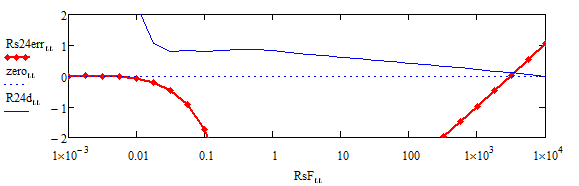
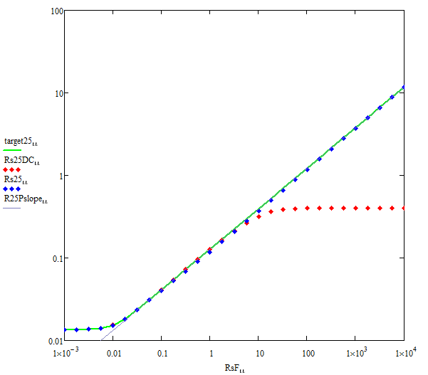
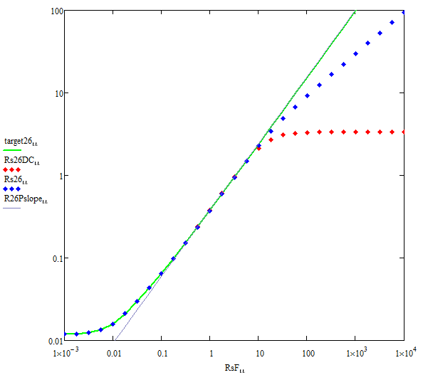
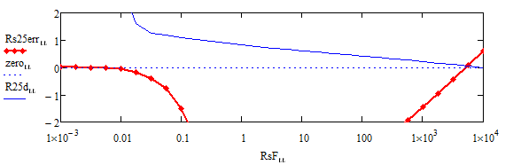
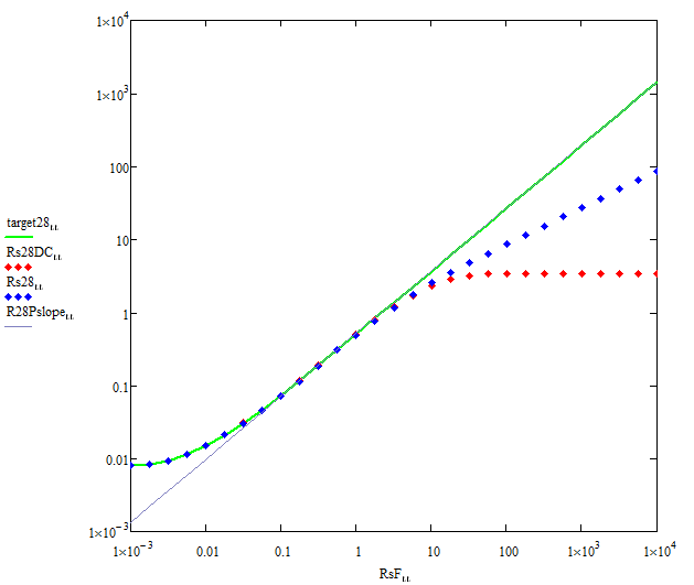
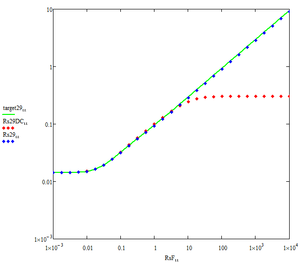
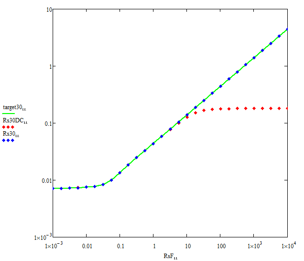
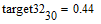
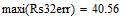
In the graphs that follow, the red and blue dots are imported data. The data was produced by atlc2 runs. SkinFix was disabled for the red dots. The green line is the expected Rs. At high frequencies it can be found by choosing a middle frequency red dot and then extending it at a slope corresponding to a square root plot.
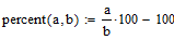
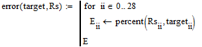
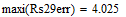
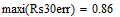
Below each Rs graph is an error graph, showing in percent how close atlc2 got to the target Rs. The graphs show that atlc2 is generally never off by more than 5 %. However this is a lie because the target is largely a guess. Furthermore, the error plots for examples 1, 2, and 3 are guaranteed to be zero since these examples were used to generate the fudge functions. The same is true for the upper frequency parts of examples 6, 7, and 8.
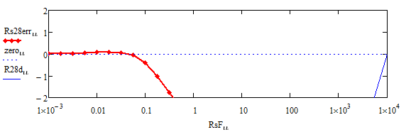
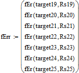
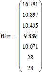
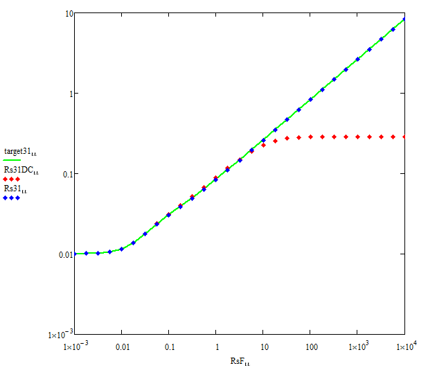
In examples 19-28, the green target line is not a square root plot. In these examples the slope of the green line is set from the slope of the RsDC plot at middle frequencies. Since atlc2 always assumes a square root plot, the errors are large. These examples show how large.
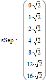
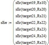
Examples 19-25 study the question "How far apart should the conductors be?"
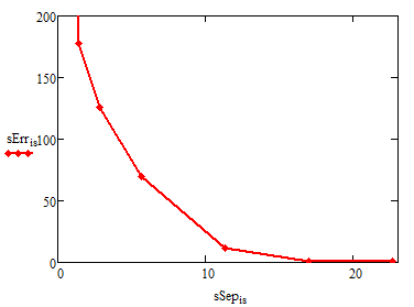
This graph is a summary of examples 19-25. It shows the error in Rs at 10000 MHz as a function of the separation between corner pixels of differing voltage. For the error to be less than 5% the spacing must be at least 14 pixels.
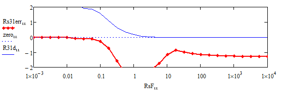
Example 32 employs pixel case H, and as a result is seriously in error at the highest frequencies. The slope at middle frequencies make clear what the truth is.
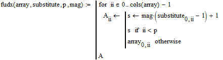
The following will create six files. Each file contains the target Rs values for one example. Atlc2 will search for the fudge function that will make its Rs results match these target values.
The values found by atlc2 for fudgeD, fudgeE, and fudgeF are valid only above about 10 MHz. Below that frequency, the plots turn wildly random. This is because the corner pixels carry so little current that their contribution is lost in the data noise and other approximations.
To fix this, the fudx function steals data from other plots. So while the functions look good, they are a complete lie at low frequency. (It doesn't matter since the corner pixel contributions are insignificant at low frequency.)
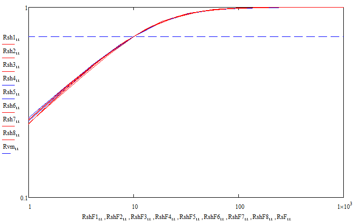
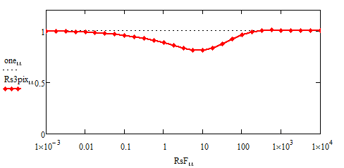
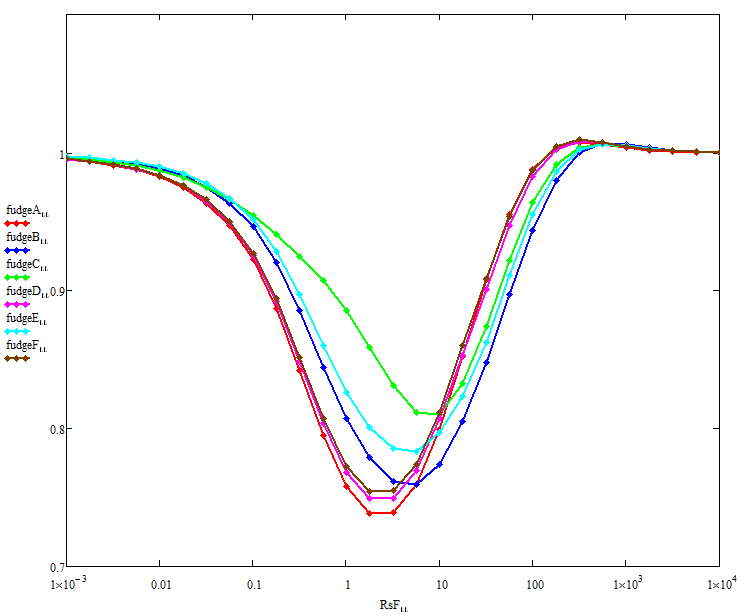
While examining the 32 examples above, I eventually noticed that the transition from middle to high frequencies (the "knee") always seemed to have the same shape. I decided to use this to compute the intercept for each plot. (It is best to stay far away from low frequency effects.) The graph below shows the first eight examples shifted so as to coincide, and showing that the knees in fact have the same shape.
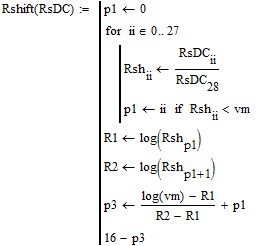
 finds how much lateral shift is necessary to make the plot cross a fixed point.
  will find the point which is 0.7 of the plot's highest value, and will shift the plot so that that point is at 10 MHz. The choice of 0.7 was somewhat arbitrary.
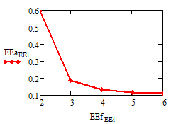
The following is a study of the effects of the "Restrict to skin depth" feature, which says " blacken all pixels deeper than M times the skin depth (where M=3), or N pixels (where N=3), whichever is greater". This study experiments with other values for M and N, determining what the average error would be compared to not using the feature.
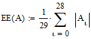
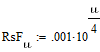
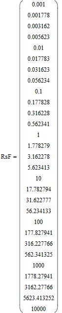
The M and N values are constants, so atlc2 had to be reassembled for each test below. Each test was at the 29 frequencies described by RsF.
My final conclusion was that 3 and 3 were the best values, because smaller values caused a sizable jump in the average error.


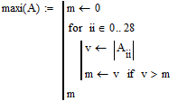
 measures the amount of lateral shift in the plot.
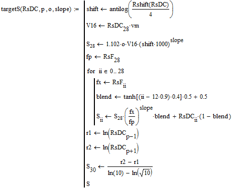

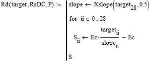
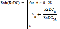
 predicts Rs given RsDC.


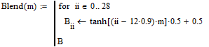


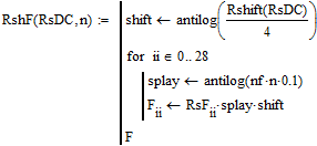
 splays the graph so that individual plots can be identified.)