9/29/20
This is the manual for
atlc2
Arbitrary Transmission Line Calculator
Current version: 1.04 9/29/20
This program was inspired by the atlc program written by Dr. David Kirkby, G8WRB.
You submit a drawing showing the cross-section
of a transmission line with any geometry.
From that, the program will use numerical methods to find Z0
and the other transmission line parameters.
Atlc2 is entirely free.
Download atlc2 for Win32 now (2.61M bytes)
Download atlc2 for Win64
now (4.36M bytes)
(The Win32 version will
run on a 64-bit Windows system. The only
advantage of the Win64 version is it allows more than 13500 equations.)
Differences
between atlc and atlc2
1. Atlc2 applies Faraday’s
Law to determine the current distribution inside the conductors. From that it calculates the inductance and
skin effect resistance. Atlc used only
the laws of electrostatics.
2. Atlc2 is well thought
out for unshielded lines, solving them rapidly and accurately. (Surrounding them with a ground shield just
slows down the program.)
3. The size of the
simulation is not related to the size of the drawing. The E field simulation is always 3200 x 3200
pixels.
4. If there is a third
conductor, it can either be pinned to ground potential or it can float to an
unforced voltage level.
5. Atlc2 is a Windows
program. Atlc was a Unix program, not
especially user friendly.
6. Atlc2 can internally
generate some simple geometries. In such
cases no drawing file is necessary.
Atlc2 will accept drawing files created for
atlc.
General
description
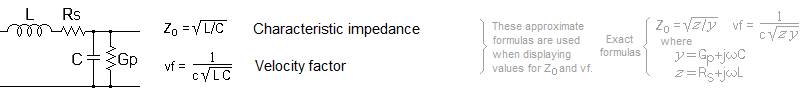
Atlc2 computes Z0, vf, L, C, Rs, Gp,
and VO for any geometry. (VO
is the offset voltage necessary for no radiation.)
There are formulas for Z0 for simple
geometries, but they are not always accurate.
If the geometry is extreme or complicated, has regions with dielectrics,
or if the skin-effect resistance is wanted, then a program like this one is
your best hope.
If used properly, atlc2 results are accurate to
1% or better. But it is not fast. It is compute intensive. Some speedups are employed that work well for
some geometries, but not others. It can
be hard to predict whether a run will take seconds or hours. Run atlc2 on your fastest computer.
Microsoft Paint is a good program for creating
the drawing, but any such bitmap editor will work. There must be no de-aliasing, so Photoshop is
out and JPEG files will not work. BMP
format is assumed but TIFF and PNG files will also work.
Normally red, green, blue, and cyan are
conductors and all other colors are insulators.
The line conductors can be any 2 of the 3 primary colors, but if all 3
appear then green is assumed to be ground.
But other color schemes are allowed. Color definitions can be changed at the
keyboard or they can be loaded from a file.
Most commonly red is +1 volt (actually +sin ωt),
blue is –1, green is 0, and cyan is varying (floating).
Unlike atlc, atlc2 requires a frequency, a
definite size, and a conductor resistivity.
But you can specify anything if they have little effect on the
results. Full red, green, and blue
(x0000FF, x00FF00, and xFF0000) are now copper.
But slight off-shades are defined for other common metals. Atlc2 has 45 predefined colors for the common
materials.
Installing
atlc2
Atlc2 is a Windows program. It will run on Window 2000 and newer. The 64-bit version is required if you need
more than 13,500 equations (unlikely).
Tryouts: atlc2 can be executed directly upon
download. It does not have to be saved
to disk.
There is no formal installation procedure. It is a single .exe file and does not require any other
files. It is not a registering program and
does not show up in the Windows list of installed programs.
You probably should create a new folder and put atlc2.exe in that folder. We shall call it the “execution folder”. It can have any name but should not be
read-only. Atlc2 will record the results
of any run that takes longer than 1 minute.
Those results go into a file called altc2
log.txt in
the execution folder.
Drawing files and any files produced by atlc2
can reside in any folder, but the open and save dialogs will always start at
the execution folder. So it is most
convenient to keep your atlc2 files there.
You may want to create a file that declares
colors as conductors or insulators, and assigns physical characteristics to
them. This file must be called MoreColors.txt and it must be in the
execution folder.
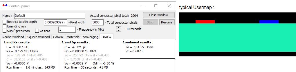
Usermap: Preparing the drawing
(De-aliasing is a blurring of edges that makes
them less jagged. But it creates
unintended colors that atlc2 will not recognize. So you must use an editor that avoids that.)
Commonly red and green are used for fully
shielded lines, such as coaxial cable.
Otherwise use red and blue. When
red and blue are both present, they are adjusted by adding VO to
both, maintaining the 2–Volt difference.
(The program searches for a VO that produces no radiation.) Green is always kept at exactly 0 volts.
The drawing can be in any folder and have any
name. But finding the file is easier if
you put it in the execution folder and give it the name Usermap YYY
ppp.bmp,
where “ YYY” is a phrase describing the drawing. YYY can be a mix of upper and lower case and
can contain spaces, but “Usermap” should be as
shown. (The open dialog will initially
filter out other files.) “ ppp” is
optional. If it is a string enclosed in
parentheses, the string will be moved to the pixel width edit box.
Example: Usermap Example 1 (.1mm).bmp
When the checkbox “Restrict to skin depth” is
checked, the program automatically blackens out conductor pixels more than
3δ from the surface, where δ is the predicted skin effect depth. (So setting the frequency too low makes the
program run longer.) (Using this feature
causes a decrease in accuracy of less than 1%.)
The pixels at the edge of the Usermap are
special. They are replicated outward
until the map is 3200 x 3200. (The four
corner pixels are doubly special. They
are replicated in two dimensions.)
Floating wires cannot carry a net current, but
they can carry local currents (eddy currents).
That is, there will be return currents in other floating pixels (so that
they sum to zero).
All +1 pixels (usually red) are electrically
connected to a voltage source. Thus they
are connected to each other. The same is
true for -1 wires (usually blue) and ground wires (usually green). But floating wires are connected to each
other only if they are exactly the same color.
So eddy currents will not link floating wires of different color.
A grounded third wire (usually green) can carry
a net current. But if it does then the stated
impedance is not a true characteristic impedance. If the ground current is more than a few %
then the impedance the program reports should be disregarded.
The standard (internally defined) colors are:
Red Green
Blue use resistivity permittivity tanδ
permeability name
███ 255 0 0
x0000FF +1 1.7241
1 1 copper
███ 0 255 0
x00FF00 0 1.7241
1 1 copper
███ 0 0 255
xFF0000 -1 1.7241
1 1 copper
███ 0 255 255
xFFFF00 float 1.7241
1 1 copper
███ 224 31 31
x1F1FE0 +1 2.62
1 1 aluminum
███ 31 224 31
x1FE01F 0 2.62
1 1 aluminum
███ 31 31 224
xE01F1F -1 2.62
1 1 aluminum
███ 31 224 224
xE0E01F float 2.62
1 1 aluminum
███ 224
31 0 x001FE0
+1 1.62 1
1 silver
███ 31
224 0 x00E01F
0 1.62 1 1 silver
███ 31
0 224 xE0001F
-1 1.62 1 1 silver
███ 31
255 224 xE0FF1F
float 1.62 1 1 silver
███ 224
0 31 x1F00E0
+1 2.44 1 1 gold
███ 0
224 31 x1FE000
0 2.44 1 1 gold
███ 0
31 224 xE01F00
-1 2.44 1 1 gold
███ 0
224 224 xE0E000
float 2.44 1 1 gold
███ 224
63 63 x3F3FE0
+1 9.71 1 1 * steel
███ 63
224 63 x3FE03F
0 9.71 1 1 * steel
███ 63
63 224 xE03F3F
-1 9.71 1 1 * steel
███ 63
224 224 xE0E03F
float 9.71 1 1 * steel
███ 224
0 63 x3F00E0
+1 11.4 1 1 tin
███ 0
224 63 x3FE000
0 11.4 1 1 tin
███ 0
63 224 xE03F00
-1 11.4 1 1 tin
███ 0
255 224 xE0FF00
float 11.4 1 1 tin
███ 24
63 0 x003FE0
+1 14.5 1 1 60/40 PbSn solder
███ 63
224 0 x00E03F
0 14.5 1 1 60/40 PbSn solder
███ 63
0 224 xE0003F
-1 14.5 1 1 60/40 PbSn solder
███ 63
255 224 xE0FF3F
float 14.5 1
1 60/40 PbSn solder
tanδ
███ 0 0
0 x000000 insul
1000000 1 0
1 vacuum
███ 255 255
255 xFFFFFF insul 1000000
1 0 1
vacuum
███ 255
202 202 xCACAFF insul 1000000
1.0006 0 1 air
███ 130
53 239 xEF3582
insul 1000000 2.07
0.00020 1 teflon
███ 255
0 255 xFF00FF
insul 1000000 2.26
0.00064 1 polyethylene
███ 255
255 0 x00FFFF
insul 1000000 2.5
0.00033 1 polystyrene
███ 239
204 26 x1ACCEF
insul 1000000 4.5
0.011 1 polyvinylchloride
███ 188
127 96 x607FBC
insul 1000000 3.3350 0.03 1
epoxy resin
███ 26
239 179 xB3EF1A
insul 1000000 4.8
0.018 1 fiberglass/epoxy PCB
███ 223
247 136 x88F7DF
insul 1000000 3.7
0.018 1 FR4 PCB
███ 142
142 142 x8E8E8E
insul 1000000 2.2
0.00090 1 duroid 5880
███ 105
105 105 x696969
insul 1000000 6.15
0.00270 1 duroid 6006
███ 220
220 220 xDCDCDC insul 1000000
10.2 0.00230 1 duroid 6010
███ 213
160 77 x4DA0D5
insul 1000000 100
0 1 Er=100
███ 100
200 255 xFFC864
insul 1000000 75
0.157 1 distilled water
███ 176
224 200 xC8E0B0
insul 1000000 3.78
0.00006 1 quartz
███ 153
255 153 x99FF99
insul 1000000 5.0
0.00540 1 glass (varies a lot)
* Atlc2 cannot presently handle ferromagnetic
materials.
The tanδ values above are rough typical
values. The program assumes tanδ is
constant. But for most materials,
tanδ varies slightly with frequency and manufacturer. (Tanδ specifies the dielectric
loss. It is used only for the
calculation of Gp.)
Best
practices
The Usermap can have any dimensions. A larger Usermap (a map with more pixels per
conductor) will run slower, but a smaller map will not represent fields or
curved surfaces as well. The gap between
conductors must never be less than 2 pixels, and accurate results usually
require a gap of at least 5 pixels.
There is no need or benefit to having empty
space around the transmission line.
(This is true for shielded and unshielded lines.) The Usermap can be the smallest map that
describes the line.
Usually the overriding goal is a Usermap with
1000 to 3000 conductor pixels, which will solve for L and Rs in a couple minutes.
Execution time rises dramatically with the conductor pixel total (roughly
the cube of the equation total). Solving
for L and Rs takes:
200 conductor pixels - 1 second on a 1.5 GHz Pentium 4
400 conductor pixels - 4 seconds on a 1.5 GHz Pentium 4
800 conductor pixels - 1.4 minutes on a 1.5 GHz Pentium 4
1600 conductor pixels - 13.0 minutes on a 1.5 GHz Pentium 4
3200 conductor pixels - 100.6 minutes on a 1.5 GHz Pentium 4
3200 conductor pixels - 7.0 minutes on a 3.33 GHz Xeon, 1 thread
3200 conductor pixels - 1.2 minutes on a 3.33 GHz dual Xeon, 12 threads
6400 conductor pixels - 9.0 minutes on a 3.33 GHz dual Xeon, 12 threads
12800 conductor pixels
- 90.0 minutes on a 3.33 GHz dual Xeon, 12 threads
25600 conductor pixels
- 14 hours on a 3.33 GHz dual Xeon, 12 threads (64-bit version)
So it is best to let the “pixels per inch” be
determined by whatever scale gets a reasonable execution time. Execution times to solve for C and Gp are more variable, but runs
can be ended early if convergence is seen.
C and Gp finds the capacitance
(and Gp) by summing the energy in the field, so some capacitance is missed if a
considerable field extends beyond the 3200 x 3200 area. Thus while Usermaps as large as 3200 x 3200
are allowed, C and Gp becomes
inaccurate if the conductors are not confined to the central 1600 x 1600
region. Ground planes and fully shielded
lines are exceptions to that.
Getting
an accurate Rs
Rs will be accurate to ±1% when the skin depth
is at least 30 times the pixel width. In
other cases, atlc2 estimates the A.C. resistance of each pixel. In these cases, Rs is generally accurate to
±5%. But this is true only if the
conductors are not too close. The
following diagram shows the minimum spacing if you want Rs accurate to 5%. A corner pixel must be at least 16 pixels
from another corner pixel of different voltage, or 8 pixels from a flat or
curved surface of different voltage.
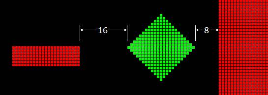
If you violate this, atlc2 will report the Rs
value using a red font as a warning. To
work around that, you will need to make a larger model (with more conductor
pixels) and then hollow it out to reduce the pixel count.
Atlc2 might be the only program anywhere that
can predict Rs within 5% for any wires with any cross-sections.
Running
atlc2
Atlc2 begins by showing one of its internally
generated examples. The normal procedure
is to click File>Open and select
the BMP file that you have prepared. You
must provide a “Pixel width” when using an external bit map. Then click Solve>Solve fully. Or File>New will select a different
internal example.
Wherever atlc2 asks for a numerical value, the
entered value can be an integer or floating point number. The numerical value can be followed by a
power-of-ten suffix in “e” form. For
example, 13e-3 would be 13 thousandths of an inch. Additional suffixes are allowed:
in (inches)
m (meters)
cm (centimeters)
mm (millimeters)
AWG (American wire gauge)
Inches are assumed if
there is no suffix.
Some keyboard command
keys are available:
U Show without E or V field
V Show the V field intensity
E Show the E field intensity
D Show the D field
intensity (where D is εE)
T Show the loss
distribution (where loss is εEtanδ)
L Show the V field as a
lines plot. (These lines are often perfect
circles.)
N Show the E field as a lines
plot (lines of force direction)
B Show both the E and V field
lines
J Show J-field, not the
Usermap (The Usermap substitutes when
the J-field is not yet found.)
H Show all fields high
intensity (employs a square root function)
S Stop solving
+ or = Zoom in
- Zoom out
] or PgUp Rescale
larger
[ or PgDn Rescale
smaller
> or Insert denser lines
< or Delete sparser lines
Enter redraw plot
&J Write the entire current map
to a text file
&V Write the entire voltage map
to a text file
(The &L, &T, &K, and &G
commands are undocumented. They are not
of general interest.)
Color definitions can
be modified using the keyboard. If the
“Show all standard colors” box is checked, the changes are to the internal
color table and persist until the program terminates. Otherwise the changes persist only until the
Usermap is changed.
MoreColors.txt
This file does not have to exist. Any text editor can be used to create it.
A sample MoreColors.txt file:
|red: green: blue:
use: Ohms: Er: tanDelta: Mu:
name:
250
20 20 +1
7.3 1 0 1
Cadmium
30 255 30
0 20.6 1
0 1 Lead
180 180 120
insul 0 6.0
0.0007 1
Mica
30 30 30
insul 0 3.5
0.0040 1 Hard rubber
100 140 170
insul 0 4
0.0030 1 Silicone
Each line in the file declares and defines one
color. All parameters must appear in
order. The parameters are:
1. Red value. (0 to 255)
2. Green value. (0 to 255)
3. Blue value. (0 to 255)
4. Function. (must be +1, –1, 0, float, or insul)
5. Resistivity in
Ohm-Centimeters. (ignored for
insulators)
6. Relative permittivity (ignored
for conductors)
7. Loss tangent
tanδ. (dielectric loss, ignored for
conductors)
8. Relative
permeability. (for future use)
9. Material name. (Everything remaining on the line is part of
this comment. It may contain blanks.)
If a color duplicates an existing color, the
new definition prevails. Atlc2 loads MoreColors.txt only once, when it
begins. Then the user can use the
keyboard to further redefine colors. The
program will hold up to 500 colors, but only 256 can appear in a Usermap.
All parameters in this file are delimited by
blanks. A tab is treated as a
blank. Consecutive blanks are treated as
one blank. A “|” character denotes a
comment, and all further characters on the line are ignored. Blank lines are allowed.
Implementation
details
Atlc2 is written in Delphi XE10 Pascal (about
8000 lines). It uses 64-bit floating
point for all calculations. The source
code will be made public in the future.
Atlc2 uses multiple threads (cores) during E
field prediction and relaxation (C and
Gp), and equation solving (L and Rs). It assumes all of the computer’s processors
are idle. The program can manage up to
64 threads. One "master"
thread parcels out work for the others, which sit in infinite loops when they have
nothing to do. So the Task Manager
graphs do not necessarily show actual work being done. Any interruption that slows down any thread
slows down them all. You should reduce
the atlc2 thread count if your system does a lot of other concurrent work. On the author's dual-Xeon workstation,
running 12 threads is about 6 times as fast as a single thread with the other
11 cores idle.
L and Rs
This part of the program works by solving
equations, one equation per conductor pixel.
The equations force the total net current to equal zero. But there are transmission lines in which
this is not true. Some geometries
(including coaxial cable) encourage an unbalanced current, which produces an
excess charge that is balanced by a virtual charge infinitely far away. Such lines will radiate radio waves at all
frequencies if nothing is done about this.
Grounding the offending conductor might be sufficient to fix this. A driver circuit that implements VO
will certainly fix it.
If there is a grounded third wire (green) then
“Ignd” gives the ground
current compared to the red current.
Analytically this number is not very useful. It is provided as a convenience. If Ignd is below 4% then it might be safely ignored. Otherwise maybe your whole approach should be
reconsidered.
Infinite plane extensions are ignored during L and Rs. Only the conductor pixels in the Usermap
contribute toward the solution.
The math used in L and Rs is described at LandRs.html. Atlc2 correctly models eddy current loss and
low frequency dispersion.
Low frequency dispersion
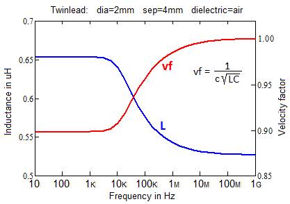
Low frequency dispersion occurs because L
changes with frequency but C does not.
C and Gp
A frequency and pixel size are not required
when solving for C and Gp. The method
used is the same as in atlc. So C is a
D.C. surface capacitance. The A.C.
capacitance is generally the same at all frequencies.
C and Gp can be thought of as a
soap-film-stretching program. Imagine
high structures (high voltage) and low structures (low voltage) with a fabric
or soapy film stretched between them.
The white V-lines (often circles) are elevation lines, like those on a
topographical map.
The method is a “relaxation algorithm” that
continuously sets the voltage at each pixel to the average of its four closest
neighbors. This will eventually
stabilize and will be a perfect solution to Gauss’s Law. How long it takes depends on how the program
initializes the array. The better the
program can predict the final field, the quicker the relaxation algorithm will
finish. Prediction uses the formula
![]() after
distributing the surface charge.
after
distributing the surface charge.
Surface charge distribution is by successive
approximations. The E field at each
surface pixel is found by summing the contributions from the charges at all the
pixels. The field component normal to
the surface predicts a new value for the charge at that pixel. About 20 iterations seems to work well.
Presently the prediction cannot guess the
effects of dielectrics. So examples with
dielectrics take longer for an accurate result.
Most other examples finish quickly.
Another slow example is any transmission line with a net charge. This will be the case if you use green
instead of blue for unshielded lines.
Such lines will radiate, and the reported Z0 is not a true
characteristic impedance. Almost
certainly you are making a mistake. If
you want to design an antenna, you need a very different kind of program.
For unshielded lines, the Usermap is extended
outward by adding pixels. These pixels
are of two different sizes. Usually the
Usermap is extended outward by 100 pixels that are the same size as the Usermap
pixels. Then the map is further extended
using pixels that are 8 times larger (256 times larger in area), until the size
of the map is equivalent to 3200 x 3200 of the Usermap pixels. Note that if you surround the conductors with
a lot of empty space (rather than use a smaller Usermap) then more of the
smaller pixels are employed, slowing down the run with probably no improvement
in the accuracy. (The region with
smaller pixels is never smaller than the Usermap.)
L and Rs versus C and Gp
Atlc2 is essentially two programs bundled together. They do roughly the same thing by two
different methods. Sometimes you need to
run both, but for other cases, one is sufficient. L and
Rs tends to be more accurate, but its execution time rises with the cube of
the conductor pixel total, which can be prohibitive. L and
Rs cannot handle multiple dielectrics.
C and Gp loses accuracy when
the conductors are close together.
(Close conductors will spike the capacitance, which a coarse grid
portrays poorly, but the inductance remains well behaved.)
C and Gp is itself two programs
bundled together: A charge-shifting
program and a relaxation program. Either
could do the whole job. The former is
usually faster, but the latter is more accurate. So C
and Gp employs both. In cases where
charge-shifting is slower, you might want to skip it, which is done by checking
the box “Skip E prediction”. Execution
time for prediction rises with the cube of the model size, while relaxation is
roughly the square.
If you must use a map too large for L and Rs, try this trick: Run C
and Gp a second time but with all permittivities
set to 1, and use the L that it reports.
Z0 = sqrt(L/C)
A
discussion of 3-wire transmission lines
Multi-wire transmission lines have multiple
characteristic impedances, none of which truly correspond to that of a 2-wire
transmission line.
Any 3-terminal linear network can be modeled as
3 impedances in either a “Y” or “delta” configuration. We shall use a “Y” to describe a 3-wire line
as seen from the end.
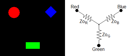
If the green wire is made to float, it will
carry no current. Upon running atlc2,
let’s designate the resulting impedance ZoGCZ
(green current zero). Two more
runs of atlc2 will give us ZoRCZ and ZoBCZ. It
is evident that:
ZoRCZ = ZoB
+ ZoG
ZoGCZ = ZoR
+ ZoB
ZoBCZ = ZoR
+ ZoG
These can be solved for ZoR,
ZoG, and ZoB:
ZoR = (ZoGCZ
+ ZoBCZ – ZoRCZ)/2 ZoG =
(ZoRCZ + ZoBCZ
– ZoGCZ)/2 ZoB =
(ZoRCZ + ZoGCZ
– ZoBCZ)/2
________________________________________________________________________
A quarter-wave directional coupler is a common
3-wire transmission line:
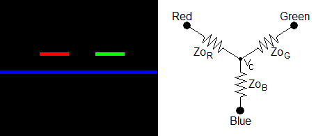
If the green wire is made to float then there
is no green current. Whatever float
voltage atlc2 reports will be equal to the center voltage, VC. Thus:
ZoB = ZoGCZ
* (Vfloat+1) / 2 ZoR = ZoGCZ – ZoB ZoG
= ZoR
ZoODD = 2 * ZoR ZoEVEN
= ZoR / 2 + ZoB
So it is possible to get a complete
characterization with a single run of atlc2.
In theory this works. In
practice, the results are often off by more than 5%. The problem is that the asymmetry results in
an unbalanced charge. The resulting
radiation for this partial result does not resemble the radiation of the
circuit used properly. L and Rs understates
the radiation, while C and Gp overstates it.
To get accurate results, make two runs that find ZoODD
and ZoEVEN directly.
Scripting
Facility
Although I added this feature for my own use,
you might find it useful.
If you enter ZZZ in the Name box and
then select File>Run Script,
atlc2 will open the file ZZZ.txt and execute the
commands it finds there. The file name
ZZZ can be a mix of upper and lower case and may contain blanks.
When the atlc2 application begins, it looks for
the file StartupScript.txt. If found, atlc2 will execute it.
A sample script file:
| A sample script file
twinlead
box 1 F
| restrict to skin depth
total 4000
separation 6mm
diameter 2mm
frequency .001
sweep frequency 25 4
The file format rules are the same as for MoreColors.txt. Only
the first 3 characters of each command name are examined. When the argument is a directory or file
name, the case and any blanks are preserved.
Otherwise the case does not matter but there must be no blanks within an
argument. Most commands are simple string
moves. Very little error checking is
performed. A detected error will abort
the script. The "Stop" button
will abort the script. No files are kept
open during solves or script execution.
Allowed
commands: (arg1, arg2, and arg3 are the command
arguments)
twinlead equivalent to File>New twinlead
square equivalent to File>New square twinlead
coaxial equivalent to File>New coaxial
pixel moves arg1 to the "Pixel
width" box. (This has no effect
unless the Usermap is from a file.)
total moves arg1 to the "Total
conductor pixels" box. (This has no
effect unless the Usermap is internally generated.)
frequency moves arg1 to the "Frequency"
box.
separation moves arg1 to the "Wire
separation" box.
diameter moves arg1 to the "Wire
diameter" box.
insulation moves arg1 to the "Insulation
diameter" box.
top moves arg1 to the "Top
distance" box.
bottom moves arg1 to the “Bottom distance”
box.
side moves arg1 to the "Side
distance" box.
skew moves arg1 to the "Vertical
skew" box.
width moves arg1 to the "Wire
width" box for square twinleads.
height moves arg1 to the "Wire
height" box for square twinleads.
center moves arg1 to the "Center
conductor diameter" box for coaxial cables.
inner moves arg1 to the "Shield
inner diameter" box for coaxial cables.
outer moves arg1 to the "Shield
outer diameter" box for coaxial cables.
box set the checkbox designated by
arg1. Arg2 should be a T or F. See note 5.
name moves arg1 to the "Name"
edit box. The case and any blanks within
arg1 are preserved.
folder designates a folder. Thereafter, all references to the execution
folder will use this folder instead.
open like File>Open. A Usermap is loaded from arg1.bmp. See note 1.
solve equivalent to Solve>Solve
fully. See notes 2 and 3.
LRS equivalent to Solve>Solve for
L and Rs. See note 2.
CGP equivalent to Solve>Solve for
C and Gp. See note 3.
sweep L
and Rs parameter sweep. arg1:
parameter. arg2: number of runs. arg3: runs per decade. See note 4.
terminate terminate atlc2.
erase erase the script file.
window set the window state for this
application. Arg1 gives the window
state: 0 - wsNormal, 1 - wsMinimized,
2 - wsMaximized, etc.
launch launch arg2 as an app (using ShellExecute). See
note 1. Arg1 gives the window state: 0 -
sw_Hide, 1 - sw_ShowNormal,
3 - sw_ShowMaximized, etc.
save write the displayed image to the
file named by the “name” box. (no
prompting)
keyboard apply each character of arg1 as a
keyboard character. (Function keys can
be entered as Fn. F8 will call another
script.)
threads use arg1 threads (cores). Arg1 can be a + or – to increment or
decrement the current setting.
beep sound the console bell (ding).
Note 1 If the first character of the file name
is a % then the % is replaced by the execution folder name. Do not follow the % with a \. (A \ will be included automatically.)
Note 2 The computed L is appended to ZZZ Inductances.txt, and Rs is appended to ZZZ Resistances.txt. These
files are cleared when the script begins.
Note 3 The computed C is appended to ZZZ Capacitances.txt, the computed Gp is appended to ZZZ Conductances.txt, and vf is appended to ZZZ VFactors.txt. These
files are cleared when the script begins.
Note 4 Arg1 can be any of these: pixel,
total, frequency, separation, diameter, insulation, top, bottom, side, skew,
width, height, center, inner, or outer.
Each refers to the same edit box as the same-name command above. See note 2.
Example:
If the frequency box contained 10 then "sweep frequency 5
2" would run L and Rs
with the frequencies 10, 31.62, 100, 316.2, and 1000 MHz.
Note 5 Specify a number for the desired
checkbox:
1 Restrict
to skin depth
2 Unending
run
3 Skip
E prediction
4 Vo
zero
10 Add
top plane
11 Add
bottom plane
12 Add
side planes
13 Insulation
vertical
14 Insulation
horizontal
15 One
wire
20 Add
floating wire
21 Add
grounded wire
30 Air
dielectric
31 Show
all standard colors
Windows
versions before XP
Early versions of Windows would not accept
blanks within file names. When atlc2
detects these versions, it will require an underscore in place of a blank. (I have no way to test this. If this detection fails, the &X command
will toggle it.)
Revision
history
Version
1.04 L=0 bug fixed. (L was always zero
in Inductances.txt)
Version
1.03 Gp bug
fixed. (Gp was
wrong in the 2v case.) The program can
now handle 64 threads.
Version
1.02 The pixel width can be specified
in the file name. The loss field is
new. The arrow keys are fixed.
Version
1.01 Control panel rescaling is new.
Version 1.00
This is the
first version I am proud of. It has no
bugs, so far as I know. If you see
anything that might be a bug, please report it to me at kq6qv@aol.com
. I will fix it quickly.
Previous
versions had problems with charge prediction that sometimes caused them to run
very slowly. This has been mostly fixed.
Some small
changes to the program:
1. A new checkbox allows E-field prediction
(charge prediction) to be skipped. This
makes the run time different, but does not change the ultimate numerical
result. E-field prediction usually
speeds up the program, but for some very large examples makes it slower.
2. Gp calculation is new. (atlc2 log.txt is affected.)
3. If you created a MoreColors.txt file, it
should be changed to include tan(delta) values.
If you do not know your dielectric's tan(delta) or don't care, specify a
0.
4. I decided to change the name of "C and
vf" to "C and Gp". This
is a purely cosmetic change.
5. Clicking on "File>Save displayed
bitmap as..." now saves the full 3200 x 3200 map, with no zooming.
6. PNG and TIFF files now work again. Saved images will have the same file format
as the Usermap.
7. C and Gp now employs up to 32 threads.
8. Rs prediction is now accurate to 5 %.
9. Rescaling is new, allowing Usermaps from
files to be resized. (It looks like
zooming, but actually changes the number of Usermap
pixels.)
10. C and Gp predicted L and Zo by assuming
vf=1. L and Rs predicted C and Zo by
assuming vf=1. Both have been changed to
make a guess about vf. The guess
averages the permittivities of all the dielectric
pixels, weighing them equally. This is
often a rather poor guess, but it is usually closer than assuming vf=1.
11. Scripting changes: The entire script file is read into RAM and
closed before the script is executed.
The "erase" command no longer terminates the script. The command "restrict" has been
replaced by "box 1", and "CVF" has been replaced by
"CGP".
"Conductances.txt" is new.
Scripts can call other scripts (key F8).
12. E-field lines is new. The line density is adjustable.
bottom